Simulations
CBM offers many methods inteded for model analysis.
Note: arguments inside brackets [ ] denote keyword arguments, for example
flux balance analysis is defined as
fba(model; [direction = "max"])
meaning you can equivalently call:
fba(model)
fba(model, "max")
fba(model, direction = "max")
- Flux Balance Analysis
- Flux Variability Analysis
- Find blocked reactions
- Synthetic Lethal Genes
- Robustness Analysis
- Find Dead End Metabolites
- Find Essential Genes
- Find Exchange Reactions
- Find Reactions From Gene
- Find Reactions From Metabolite
- Gene Deletion
- Knockout Genes
- Knockout Reactions
- Print Reaction Formula
- Reaction Info
Flux Balance Analysis
fba() is a mathematical method for simulating metabolism in genome-scale reconstructions of metabolic networks, by optimizing the network w.r.t (usually) the reactions responsible for the organisms growth:
fba(model; [direction = "max", objective = 0])
directionmay be either"max"or"min"objectivemay be either an integer index or reaction name as it appears inmodel.rxns
Example
To maximize the default objective function:
julia> fba(model)
FBAsolution:
       obj::  0.873922
         v::  95 element-array
     slack::  72 element-array
    rcosts::  95 element-array
   success::  Optimal
      info::  SolverInfo("glpk","GLP_OPT")
To maximize “ADK1”:
julia> fba(model, objective = "ADK1")
FBAsolution:
       obj:: 166.610000
         v::  95 element-array
     slack::  72 element-array
    rcosts::  95 element-array
   success::  Optimal
      info::  SolverInfo("glpk","GLP_OPT")
To maximize the reaction number 14:
julia> fba(model, objective = 14)
FBAsolution:
       obj:: 11.104242
         v::  95 element-array
     slack::  72 element-array
    rcosts::  95 element-array
   success::  Optimal
      info::  SolverInfo("glpk","GLP_OPT")
To minimize, use:
julia> fba(model, "min")
FBAsolution:
       obj::  0.000000
         v::  95 element-array
     slack::  72 element-array
    rcosts::  95 element-array
   success::  Optimal
      info::  SolverInfo("glpk","GLP_OPT")
or fba(model, objective = "min")
Where
sol.objthe objective valuesol.vrepresents the solution vectorsol.slackrepresents the slacksol.rcostsrepresents the reduced costssol.infodetails solver information
Flux Variability Analysis
Returns the minimum and maximum flux of every reaction in the model
Note: This method may run in parallel
fva(model::Model, [optPercentage = 1, flux_matrix = false])
optPercentage: Fix the lower bound of the biomass reaction (or objective reaction) to a fraction of its maximum possible value.flux_matrix: In addition to minimum and maximum fluxes, return the entire solution flux for every reaction.
Example
To calculate the minimum and maximum flux values of every reaction with biomass fixed at 50% of its maximum value:
minFlux, maxFlux = fva(model, 0.5)
To calculate the flux values of every reaction for every reactions minimum flux and maximum flux, call:
minFlux, maxFlux, minFluxArray, maxFluxArray = fva(model, 1, true)
Find blocked reactions
Locate every reaction that is constrianed to zero flux in every case:
blocked_reactions = (model::Model, [tolerance::Number = 1e-10])
Where tolerance represents how close to absolute 0.0 the reaction flux must lie
Example
For ecoli core:
julia> find_blocked_reactions(model)
8-element Array{Any,1}:
 "EX_fru_e"
 "EX_fum_e"
 "EX_gln__L_e"
 "EX_mal__L_e"
 "FRUpts2"
 "FUMt2_2"
 "GLNabc"
 "MALt2_2"
Synthetic Lethal Genes
Check the model for essential genes, conditionally essential genes and non-essential genes
Returns a SLG type, which contains the fields ess, cond_ess and non_ess,:
synthetic_lethal_genes(model, cutoff = 0.1, num_runs = 100)
where cutoff represents the minimum biomass flux as a fraction of the wild-type flux.
num_runs indicates how many times the algorithm runs, higher number gives better results, but takes longer.
Example
To find essentiality with biomass fixed at 0.1 in 200 runs:
julia> slg = synthetic_lethal_genes(model, 0.1, 200)
run 200 of 200 Number of conditionally essential genes found: 115

Type: SLG
     Field                  Contains    Size
       ess                Essential:       7
  cond_ess    Conditional Essential:     115
   non_ess            Non-Essential:      15
ess, essential genes
Those genes, that if disabled, make biomass production ratio to the wild type drop below 10%. The field slg.ess is a Dict() containing the gene indices and the resulting biomass production after their deletion
cond_ess, conditionally essential
Those genes, that if disabled along with some other genes will make the biomass production ratio to the wild type drop below 10%. The field slg.cond_ess is a Dict() containing the conditionally-essential genes and all the gene-combinations that were checked that reduced the biomass below 10%.
Example
^^^^^^^ entry in this dictionary may be
90 => Any[Any[89,74,12,79,67], Any[92,95,67]]
meaning that disabling gene 90 along with either genes 89,74,12,79,67 or 92,95,67, brought the biomass below 10%
non_ess, non-essential genes
Genes that never have the effect of making the biomass production ratio to the wild type ratio drop below 10%. This is an array containing the indices of the genes that never brought the biomass below 10%
Robustness Analysis
Perform a robustness analysis for any number of fixed reactions, specified by indices or reaction names:
solution = robustness_analysis(model, reactions, [objective = 0, pts = [], direction = "max"])
The method can either be called with reaction names or with reaction indices.
objectivereaction can be chosen, either as the reaction name, such as"BIOMASS_Ecoli_core_w_GAM"or as an index, such as13. If left blank it defaults to the default objective of the modelptsis an array used to specify how many points are tested for each reaction, if left blank, it creates 20 points for each reaction
** direction``** represents the optimization direction, either ``"min" or "max" which is the default.
The function returns a type Robustness which has fields
resultwhich the flux values for the objective function at every point checkedreactions, the indices of the reactions (in case you forgot)rangesarrays with the flux value at every point for every checked reaction
The methods range(), getindex and size() can be used with the type, see below for examples of these methods
Example
Robustness analysis for “ACONTb” at 10 points
To see how the biomass of e_coli_core behaves if the flow of "ACONTb" is fixed at 10 different points between its minimum and maximum:
julia> robust_sol = robustness_analysis(model, ["ACONTb"], "BIOMASS_Ecoli_core_w_GAM", [10])
Robustness Analysis
                      result :     (10,) Array
                      ranges :
                              reaction :          range:
                                     5 :      (0.0,20.0)
We see that "ACONTb" (reaction number 5) has a minimum flux of 0.0, and maximum flux of 20.0.
result: To view the objective flux values type robust_sol.result or robust_sol[:]:
julia> robust_sol.result
10-element Array{Float64,1}:
 0.0
 0.840743
 0.862473
 0.87021
 0.786928
 0.629543
 0.472157
 0.314771
 0.157386
 0.0
ranges: To view the range of flux values "ACONTb" is fixed at, type ``robust_sol.ranges:
julia> robust_sol.ranges
1-element Array{Array{Float64,1},1}:
 [0.0,2.22222,4.44444,6.66667,8.88889,11.1111,13.3333,15.5556,17.7778,20.0]
range(): This method can be used to find where the objective function (the biomass) lies inside a range.
To see for which points the biomass lies between 0.3 and 0.7 type:
julia> range(robust_sol, 0.3, 0.7)
3-element Array{Tuple{Int64},1}:
 (6,)
 (7,)
 (8,)
so when "ACONTb" is fixed at either 6, 7 or 8, the biomass will have a flux in that range
getindex(): To view the biomass flux at point 6:
julia> robust_sol[6]
0.6295425429111932
and to plot (if Plots.jl is installed):
plot(robust_sol.ranges[1], robust_sol[:])
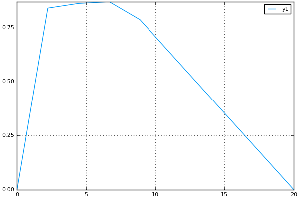
Robustness analysis for “GLUSy” and “PGM”, both at 20 points
To see how the biomass of e_coli_core behaves if the flow of "GLUSy" and "PGM" is fixed at 20 different points:
julia> robust_sol = robustness_analysis(model, ["GLUSy", "PGM"], "BIOMASS_Ecoli_core_w_GAM", [20,20])
Robustness Analysis
                      result :   (20,20) Array
                      ranges :
                              reaction :          range:
                                    55 :    (0.0,166.61)
                                    77 :    (-20.0,-0.0)
We see that "GLUSy" (reaction 55) has minimum value of 0.0 and maximum of 166.61, while "PGM" minimum is -20.0 and maximum 0.0
range(): To see for which points the biomass lies between 0.3 and 0.32 type:
julia> range(robust_sol, 0.3,0.32)
6-element Array{Tuple{Int64,Int64},1}:
 (16,10)
 (14,11)
 (10,12)
 (11,12)
 (4,13)
 (5,13)
getindex(): To view the biomass flux at point (14,11):
julia> robust_sol[14,11]
0.30173110378482915
To plot the 3D surface of the matrix of fluxes, robust_sol[:,:], do (if Plots.jl is installed):
surface(robust_sol[:,:])
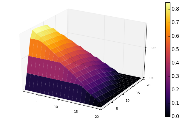
Robustness analysis for reactions 5, 22 and 76
To see how reaction 13 (biomass reaction) behaves is reactions 5 ("ACONTb"), 22 ("EX_akg_e") and 76 ("PGL") are all fixed in 20 different points:
julia> robust_sol = robustness_analysis(model, [5,22,76], 13, [20,20,20])
Robustness Analysis
                      result : (20,20,20) Array
                      ranges :
                              reaction :          range:
                                     5 :     (-0.0,20.0)
                                    22 :      (0.0,10.0)
                                    76 :      (0.0,60.0)
All the reactions have a minimum flux of 0.0. Reaction 5 has a maximum flow of 20.0, reaction 22 has a maximum of 10.0 and reaction 76 has a maximum flow of 76.0
getindex(): To view the biomass flux at point at all points for reaction 5, while reaction 22 and 76 are fixed at their maximum:
julia> robust_sol[:,20,20]
20-element Array{Float64,1}:
 0.0
 0.0
.
.
.
 0.0
 0.0
Find Dead End Metabolites
Return those metabolites that are only produced and only consumed:
find_deadend_metabolites(model, [lbfilter = true])
By default, those metabolites with a positive lower bound are filtered out of the results
Example
julia> idx = find_deadend_metabolites(model)
5-element Array{Int64,1}:
 30
 32
 37
 49
 60
Find Essential Genes
Return a list of those genes, which would, if knocked out, bring the objective flux beneath that
specified by min_growth
essential = find_essential_genes(model, min_growth)
Example
Find those genes that would bring biomass production beneath 0.01:
julia> find_essential_genes(model,0.01)
2-element Array{String,1}:
 "b2416"
 "b2415"
Note that min_growth represents the actual growth, not a percentage of the wild-type growth. For min growth of 0.1%, do:
julia> find_essential_genes(model,0.001 * fba(model).f)
2-element Array{String,1}:
 "b2416"
 "b2415"
Find Exchange Reactions
Return either the indices or names of the exchange reactions in the model:
find_exchange_reactions(model, [output = "index"])
outputcan be eitherindexorname
Example
julia> find_exchange_reactions(model, "name")
20-element Array{String,1}:
 "EX_ac_e"
 "EX_acald_e"
 "EX_akg_e"
 "EX_co2_e"
 "EX_etoh_e"
 "EX_for_e"
 "EX_fru_e"
 "EX_fum_e"
 "EX_glc__D_e"
 "EX_gln__L_e"
 "EX_glu__L_e"
 "EX_h_e"
 "EX_h2o_e"
 "EX_lac__D_e"
 "EX_mal__L_e"
 "EX_nh4_e"
 "EX_o2_e"
 "EX_pi_e"
 "EX_pyr_e"
 "EX_succ_e"
Find Reactions From Gene
Return the indices of those reactions affected by a specified gene, specified by name or index, and output can be either “index” or “name”:
find_reactions_from_gene(model, gene, [output = "index"])
outputcan be eitherindexorname
Example
To find the indices of those reactions affected by gene “s0001”:
julia> find_reactions_from_gene(model, "s0001", "index")
5-element Array{Int64,1}:
  2
 14
 58
 69
 70
Example
Find the names of the reactions affected by gene number 3 in model.genes:
julia> find_reactions_from_gene(model, 3, "name")
5-element Array{String,1}:
 "ACALDt"
 "CO2t"
 "H2Ot"
 "NH4t"
 "O2t"
Find Reactions From Metabolite
Find those reactions a specified metabolite appears in, the metabolite either specified by its name as it appears in model.mets, or by its index:
find_reactions_from_metabolite(model, metabolite, [output = "index"])
outputcan be eitherindexornameorformula
Example
To find the indices of those reactions where “cit_c” appears:
julia> find_reactions_from_metabolite(model, "cit_c")
2-element Array{Int64,1}:
  4
 15
Gene Deletion
Perform single- or double-gene deletion on the model, or the n-th gene deletion:
gene_deletion(model, n)
Lets do a double gene deletion:
gene_del_sol = gene_deletion(model,2)
gene_deletion() returns a GeneDeletion object, which containts the fields r_f, r_f and g_f
r_f, stands forreaction_flux, and contains aDict()where the keys are combinations of reaction indices, and the corresponding flux-value as a fraction of the wild type, if these reactions are disabled, for example:julia> gene_del_sol.r_f Dict{Any,Any} with 684 entries: Any[52,90] => 0.982133 Any[55,81] => 1.0 Any[57,95] => 0.0 Any[2,14,70,81] => 0.241601 #knocking out reactions 52 ("GLNabc") and 90 ("SUCOAS") #brings the biomass to 98% of its maximum
r_g, stands forreaction_genecombo, and contains aDict()where keys are reaction combinations, and the values are arrays of the gene combinations that result in the knockout of the reaction combination:julia> a.r_g Dict{Any,Any} with 684 entries: Any[57,65] => Any[String["b2029","b1479"]] Any[8,71,92] => Any[String["b0116","b1602"],String["b0116","b1603"]] Any[60,75] => Any[String["b4015","b2926"]] # so knocking out either both "b0116" and "b1602", or both "b0116" and "b1603" # will knock out reactions 8 ("AKGDH"), 71 ("PDH") and 92 ("THD2") # but knocking out reactions 57 ("GND") and 65 ("ME1") can only be achieved # by knocking out "b2029" and "b1479"
g_f, stands forgene_flux, and comtains aDict()where keys are gene-combinations and the values are the flux-value as a fraction of the wild type, if the gene-combination in the key is knocked out:julia> a.g_f Dict{Any,Any} with 9453 entries: String["b0809","b3952"] => 1.0 String["b2280","b2458"] => 0.242199 # knocking out "b0809" and "b3952" wont have any effect # "b2280" and "b2458" brings the biomass flux down to 24% of the wild-type flux
Knockout Genes
Perform fba after knocking out a set of genes, specified either by indices or their names.
Return a GeneKnockout type with fields growth, flux, disabled and affected:
knockout_genes(model, gene_index)
knockout_genes(model, gene_name)
Example
To view the effect of knocking out genes ,”b1849” (gene 4), “b3731” (gene 16) and “b0115” (gene 99):
julia> knockout_genes(model, ["b1849", "b3731", "b0115"])

Type: GeneKnockout
                        Fields
                        growth :                      0.374230
                          flux :              Array{Float64,1}
                      disabled :                       [12,71]
                      affected ::
                                               gene:      reactions:
                                          gene_016 :            [12]
                                          gene_004 :             [3]
                                          gene_099 :            [71]
knockout_genes() returns a GeneKnockout type, which has the fields growth, flux, disabled and affected
growthis simply the biomass reaction (or the objective reactions) flux after the knockout of the genesfluxis the entire solution vector, containing the flux values of every reaction in the modeldisabledis an array containing the indices of the reactions that get disabled, reaction12is"ATPS4r"and reaction71is"PDH"affectedis aDict(), where the keys are the gene names and values are arrays of the reactions that are affected but not necessarily knocked out by that gene
Knockout Reactions
An algorithm that attempts to return those genes that can be knocked out to disable a specified set of reactions
The reactions can be specified as a single reaction by name or index, or as an array of multiple names or indices:
knockout_reactions(model, reaction)
knockout_reactions(model, reactions)
Example
See if “ACONTb” (reaction 5) can be disabled:
julia> knockout_reactions(model,5)
1-element Array{Array,1}:
 [8; 7]
So knocking out genes 8 and 7 will disable reaction 5
Print Reaction Formula
Print the formula for a specified reaction specified by name or string:
print_reaction_formula(model, reaction)
Example
To print the formula for “ACONTb” (reaction 5):
julia> print_reaction_formula(model,"ACONTb")
        1.0 acon_C_c + 1.0 h2o_c  -> 1.0 icit_c

# or

julia> print_reaction_formula(model,5)
        1.0 acon_C_c + 1.0 h2o_c  -> 1.0 icit_c
Reaction Info
Print out the information for a reaction specified by name or string:
reaction_info(model, reaction)
Example
View reaction information for “ACONTb” (reaction 5)
julia> reaction_info(model, "ACONTb") # or reaction_info(model, 5)


 Reaction Name:     Aconitase (half-reaction B, Isocitrate hydro-lyase)
   Reaction ID:                                                  ACONTb
   Lower Bound:                                                 -1000.0
   Upper Bound:                                                  1000.0
     Subsystem:                                       Citric Acid Cycle
-----------------------------------------------------------------------
     Metabolite    Coefficient
       acon_C_c           -1.0
          h2o_c           -1.0
         icit_c            1.0

----------------------------------
b3115  ||  b2296  ||  b1849